
So what exactly is deep learning, anyway? The phrase is fairly vague and means different things to different people depending on who you talk to. First, though, it’s good to have a basic understanding of typical machine learning tasks and pipelines to understand how deep learning is different.
Machine learning broadly is the task of modelling data, usually with some kind of numerical or statistical model. The first key distinction between machine learning tasks is between supervised and unsupervised learning:
Supervised learning encompasses algorithms for function approximation. Given a dataset \(X\) and a function \(f\) that takes elements of the dataset and produces output \(y = f(x)\), learn a function \(h\) such that \(h(x) \approx f(x)\).
This “labelling” function \(f\) can be obvious, like trying to predict the price of a car from attributes of the car like the make, model, year, mileage, condition, etc. In this case the true function \(f\) is the process a car salesman goes through to put a price on a car given those attributes. We are trying to create an approximate function \(h\) that takes the same attributes and assigns a similar price.
For some tasks it can be more opaque, like predicting today’s weather from yesterday’s weather. In the case of the weather, there is an underlying physical process but it is not a clear function that only takes as input the past day’s weather. In reality, the weather is determined by a function (the unfolding of the laws of physics) acting on a set of data (the physical conditions of our planet).
In the case of weather prediction, the physical conditions of the planet are what’s known as a latent variable or hidden variable. They are not fully observed or recorded but do affect the outcome. Our model can try to account for these variables or simply circumvent them. In either case we are trying to build an approximation of a function that doesn’t actually exist, we simply assume it does. There’s a lot of things like that in machine learning. Don’t let it bother you too much!
There is often a distinction drawn between classification and regression tasks in supervised learning:
It’s pretty confusing that both of those example algorithms have “regression” in their name, huh? There are more complicated or mixed tasks as well that involve predicting both discrete and continuous variables. We’ll worry about those later.
In unsupervised learning there are no “labels”, there is only data. Typically unsupervised learning assumes the data is drawn from some statistical distribution or generating function. Tasks in unsupervised learning involve estimating the distribution or function the data is drawn from, learning to represent the data in a different way (usually by transforming the attribute space), or finding groupings of related data points based on the similarity of their attributes.
K-means clustering is a common technique for clustering data based on similarity of attributes. Data points are clustered into groups based on their distance from each other in attribute space according to some metric. The algorithm for K-means is an example of iterative expectation-maximization (EM) algorithm for finding a local maximum of a latent-variable model.
The k-means algorithm assumes:
First k-means randomly initialzes cluster centroids. Then the algorithm alternates between expectation and maximization steps:
Expectation: assign data to clusters based on distance to nearest centroid. Each data point is assigned to the cluster of the nearest centroid by some given distance metric (often, but not always, \(L_2\)) distance.
Maximization: centroids are updated based on the data that belongs to their cluster. Typically this is done by assigning the centroid to be the mean of the data points assigned to that cluster (hence the “means” in k-means).
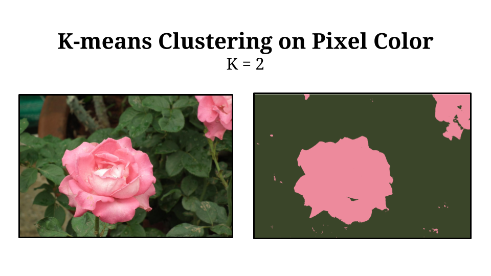
K-means clustering can be a useful tool for analyzing data sets, discovering patterns, and leveraging those patterns to accomplish some task. For example, k-means clustering on the color values of pixels in an image separates pixels into clusters based on visual similarity, giving a segmentation mask that groups visually similar elements. These elements may correspond to objects or continuous structures.
Machine learning relies on data. A data point is a collection of attributes. These attributes can be:
Machine learning algorithms usually want data in a particular format. For example, decision trees partition the data into discrete categories to make predictions thus can handle discrete attributes on their data. However, logistic regression multiplies the data attributes by a weight matrix to make predictions thus the input data should be continuous.
If we want to perform logistic regression on a data set that has discrete attributes we need to encode them somehow. One possibility is one-hot encoding. One-hot encoding converts a single, discrete attribute with \(n\) different possibilities into a binary vector with \(n\) elements.
If the cars in our dataset can be “black”, “green”, “blue”, or “red”, a one-hot encoding of this attribute would assign a black car the vector \([1,0,0,0]\), a green car the vector \([0,1,0,0]\), etc.
One-hot encoding is an example of feature extraction. Feature extraction is the process of taking raw data and converting it into useable and useful attributes for a machine learning model. Most machine learning algorithms rely heavily on feature extraction. K-means clustering needs data attributes to be in a metric space where we can compute distances. Logistic regression needs continuous data. Bayes networks assume that data attributes are conditionally independent from each other. Each of these restrictions can be addressed by extracting the right features in the right way from raw data.
Hand-designed feature extraction can be very powerful but also very tedious. Deep learning encompasses a set of algorithms that process (relatively) raw data instead of curated features. These algorithms learn to extract features from the raw data and then use those features to make predictions.
Typically deep learning is:
This is very exciting for machine learning practitioners. Typically the difference between a good and bad machine learning model comes down to the features the model uses. Good features = good model, or, as they say, “garbage in, garbage out”. Deep learning offers a different path, instead of trying to find what features make a good model, let the model learn and decide for itself.
So far deep learning has been most successful with data that has some inherent structure and the algorithms take advantage of that structure. Images are composed of pixels and nearby pixels are statistically more related to each other than far away pixels. Natural language is a string of words where future words depend on past words. Sound is a waveform composed of oscillations at different frequencies with those frequencies changing over time. These are the domains where deep learning (currently) works well.
In domains with less structure (for example, diagnosing an illness based on a patient’s symptoms) there are many algorithms that outperform neural networks or deep learning. For those tasks you are much better off using gradient-boosted decision trees or random forests.
The learning part of machine learning means automatically adjusting the parameters of a model based on data. Machine learning algorithms optimize the model parameters to give the best model performance for a data set. To optimize our model we first need a way to measure the performance of a model.
A loss function describes the performance of a model and a particular set of parameters on a dataset. In particular, it measures how badly the model performs, or how far away from correct the model’s predictions are. There are many options for loss functions but one common one is \(L_2\) loss or mean squared error.
MSE or \(L_2\) loss measures the squared distance from the models predictions compared to the ground truth over a dataset. Formally, given a dataset of paired inputs and labels \(X = (x_i, y_i)\), a model \(m\), and model parameters \(\theta\), the \(L_2\) loss is given by:
\[L_2(X, m, \theta) = \frac{1}{n} \sum_{i = 1}^n (y_i - m_\theta (x_i))^2\]In other words, we run our model \(m\) with parameters \(\theta\) on every example to obtain output \(m_\theta (x_i)\). We then take the squared distance of that prediction from the ground truth \(y_i\). We average all those errors over the full dataset.
Now that we have a way to measure how bad our model performs we want to make this term as small as possible. We usually don’t want to change our model or our dataset (that’s called cheating) but we can change our model parameters. In other words we want to find:
\[\mathrm{argmin}_\theta [L_2 (X, m, \theta) ]\]In plain english, we want to find the values \(\theta\) that minimize our \(L_2\) loss. Read on for how we can do that!
Optimization just means that given an objective function \(f\) we want to find the inputs \(x\) that give us the best output. This means finding extrema in the function output, either minima or maxima. These extrema come in two varieties, local and global.
The global minimum of a function is the point \(x\) such that the output of \(f\) is lower at \(x\) than any other point:
\[\forall_y : f(x) \le f(y)\]A local minimum of a function is a point \(x\) such that in a neighborhood \(\epsilon\) distance around \(x\), the output of \(f\) is lower at \(x\) than at any point in the neighborhood:
\[\exists_{\epsilon > 0} \forall_y: d(x,y) < \epsilon \implies f(x) \le f(y)\]The definitions are similar for global/local maxima.
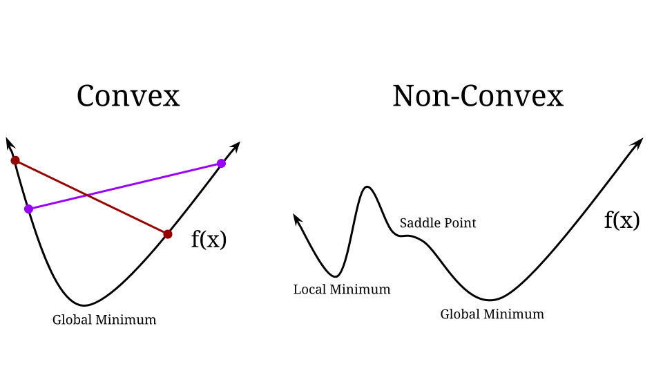
A convex function is a function where you can draw a line between any two points on the graph of the function and that line will lie above the graph. For a convex function, any local extrema is guaranteed to be the global extrema. This makes optimization a lot easier, if we find any good answer we know it’s actually the best answer. Unfortunately for neural networks we are optimizing non-convex functions.
A non-convex function doesn’t have this cup shape. There can be multiple local minima and maxima, there may be saddle points. Algorithms for non-convex optimization get stuck in local minima and have fewer guarantees about the answer they produce. Oh well, we must forge ahead anyway!
If you remember all the way back to calculus, you can tell a lot about a function by taking it’s derivative. In particular, when a function’s derivative is zero that means it’s either at a local minimum, local maximum, or a saddle point. We like local minima and local maxima and we’ll just hope for now that we don’t get stuck at a saddle point (there’s an ongoing debate in the ML community about how much saddle points matter).
Consider a simple quadratic equation. The zero crossing of the derivative shows us where a local minimum is on the function. This function is convex so we know the local minimum is a global minimum:
For some functions we may have multiple local extrema. For example \(f(x) = \sin(x)\) we have \(f'(x) = \cos(x)\) and every zero crossing of the periodic cosine function is a local minimum or maximum of the sine function.
So to optimize a function all we have to do is find where it’s derivative is zero. This might be pretty easy, consider our quadratic function:
\[f(x) = 2x^2 + .5x - 2\]In this case we just take the derivative:
\[\frac{d}{dx}f(x) = 4x + .5\]and finally set the derivative equal to zero and solve for \(x\):
\[\begin{align} 4x& + .5 = 0 \\\\ 4x& = -.5 \\\\ x& = -.125 \end{align}\]Algebraic functions (functions that are just composed of addition, subtraction, multiplication, division, and raising to a power) are often easy to solve. Transcendental functions, or non-algebraic functions, can be a bit trickier. Consider \(f(x) = e^{-x} + x^2\). We can take the derivative of this function and try to set it equal to zero:
\[\begin{align} \frac{d}{dx} f(x) &= -e^{-x} + 2x \\ 0 &= -e^{-x} + 2x \\ e^{-x} &= 2x \\ \end{align}\]But we run out of tools to solve for \(x\). But there is a zero crossing of the derivative, somewhere around \(x \approx .351734\). So how do we find it?
While there may be no closed-form solution to find the local minimum, the derivative can still be useful. The derivative tells us about the local structure of \(f(x)\):
So if we want to minimize our function we just have to move in the opposite direction of the derivative. If the derivative is positive we make \(x\) smaller. If it’s negative we make \(x\) bigger. Assuming our change to \(x\) is sufficiently small this will make \(f(x)\) go down at least by a little bit. Once we have made a change to \(x\) we can re-evaluate our derivative and see what to do next.
For example if we start at \(x = -.5\):
Say we increase every step by \(.25\)
| \(x\) | \(f(x)\) | \(f'(x)\) | Direction to move |
|---|---|---|---|
| -.5 | 1.8987 | -2.6487 | Increase \(x\) |
| -.25 | 1.3465 | -1.7840 | Increase \(x\) |
| 0 | 1 | -1 | Increase \(x\) |
| .25 | .8413 | -.2788 | Increase \(x\) |
| .5 | .8563 | .3935 | Decrease \(x\) |
We haven’t found our precise local minimum but we do know that \(f'(x)\) crosses zero somewhere between \(.25 < x < .5\). That’s pretty good! But we can do better.
Instead of moving by a constant amount every time we can move based on the magnitude of the derivative. For example, when the derivative magnitude is large we might want to move further and when the derivative is smaller we will move less. This way, if our function is smooth the example, as we get closer to the minimum we will move by smaller increments to get a better estimate.
However, before we were moving by \(.25\) every step and our smallest derivative magnitude was \(.2788\) so if we just move by the amount of the derivative we will still move too much! So we will move based on our derivative but scaled by some value.
We are finally ready for our non-convex, iterative optimization algorithm. We have some value for our function input \(x\) and at every time step we will simply move in the opposite direction of the derivative by an amount based on the magnitude of the derivative and scaled by some amount \(\eta\), called the learning rate.
We’ve been talking about derivatives, what’s this gradient thing? The gradient is sort of like a generalization of the derivative to multiple dimensions. For a function that takes multiple inputs the gradient gives the partial derivatives of that function with respect to each of the inputs. Formally:
\[\nabla f(\mathbf{x}) = [\frac{d}{d x_1} f(\mathbf{x}), \frac{d}{d x_2} f(\mathbf{x}),\frac{d}{d x_3} f(\mathbf{x}), \dots ]\]Like the derivative, the gradient of a function points in the direction of steepest ascent of the function. Therefore if we want to minimize a function we can move in the direction opposite the gradient, hence gradient descent!
Values for \(\eta\) can vary greatly depending on the problem domain or function. In neural network optimization typical values range from \([0.00001 - 0.1]\).
With some assumptions about the function being well behaved and the learning rate being sufficiently small, gradient descent is guaranteed to converge to a local minimum. However, it is not necessarrily a global minimum and depending on the initialization and function multiple runs can converge to different local minima.
For linear regression our model fits a line to a set of data: \(m(x) = ax + b\). In this case our model parameters \(\theta = \{a, b\}\). We can use our previously discussed loss function \(L_2\) to optimize this model:
\[L_2(X, m, \{a, b\}) = \frac{1}{n} \sum_{i=1}{n} (y_i - (ax + b))^2\]At every step we will update based on the gradient of the loss:
\[\begin{align} \nabla L_2(X, m, \{a, b\}) &= [\frac{d}{d a} L_2(X, m, \{a, b\}),\frac{d}{d b} L_2(X, m, \{a, b\}) ] \\ &= [\frac{d}{d a} \frac{1}{n} \sum_{i=1}^{n} (y_i - (ax_i + b))^2 ,\frac{d}{d b} \frac{1}{n} \sum_{i=1}^{n} (y_i - (ax_i + b))^2 ] \\ &= [\frac{d}{d a} \sum_{i=1}^{n} (y_i - (ax_i + b))^2 ,\frac{d}{d b} \sum_{i=1}^{n} (y_i - (ax_i + b))^2 ] \\ &= [\sum_{i=1}^{n} 2 (y_i - (ax_i + b)) \frac{d}{d a} -(ax_i + b) ,\sum_{i=1}^{n} 2 (y_i - (ax_i + b)) \frac{d}{d b} -(ax_i + b) ] \\ &= [\sum_{i=1}^{n} -2 (y_i - (ax_i + b)) x_i ,\sum_{i=1}^{n} -2 (y_i - (ax_i + b)) ] \\ \end{align}\]Let’s define \(h_i = ax_i + b\) to be the output of our model. Then we can look just at how we would update the biases of our model:
\[\frac{d}{d b} L_2 = \sum -2 (y_i - h_i)\]Since we are subtracting our gradient this means our update would look like:
\[b = b + \eta \sum 2 (y_i - h_i)\]This makes sense, if our model consistently predicts too small of values than \(\sum 2(y_i - h_i)\) will be negative and we will increase our bias. If our model predicts too large of values the sum will be negative and we will lower our bias.
The logic is similar for updating parameter \(a\) except the error our model makes is multiplied by the input \(x\). This makes sense, if the model predicts too small a value the parameter \(a\) should increase if \(x\) is positive and decrease if \(x\) is negative.
Classification algorithms assign class labels or probabilities to data instead of real-value output but they function very similarly with regards to training and testing. Binary classification is the simplest classification task, the label is just a single bit, either the data point is a positive or negative example of some particular class.
Consider the following example dataset:
| x | y | label |
|---|---|---|
| 1 | 2 | 1 |
| 2 | 3 | 1 |
| 3 | 4 | 1 |
| 2 | 1 | 0 |
| 3 | 1 | 0 |
| 4 | 3 | 0 |
Notice that when \(x < y\) the label is 1 and when \(x > y\) the label is 0. This data is linearly separable with many functions but one example would be the line defined by \(y = x\). The points that lie above this line are positive examples and the points below are negative.
In general, a linear classifier learns a model of the data that separates it based on a line (or hyper-plane in more dimensions). The model uses a function \(f\) and learns a set of weights \(w\) to make predictions where the output of the model is the probability that a data point is positive for the label:
\[\Pr( \mathrm{label} | x) = f(w \cdot x) = f(\sum_i w_i x_i)\]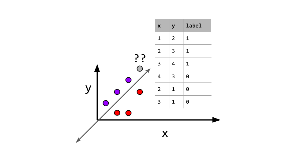
This function \(f\) can take many forms. one is simply a thresholding function: \(f(x) = \begin{cases} 1 &\text{if } x > 0\\ 0&\text{otherwise} \end{cases}\) In our example dataset one linear classifier would be a thresholding function at \(0\) with learned weights \([-1, 1]\). Given a new data point, say \([4,5]\) the model takes the dot product of the input with weights and applies the threshold:
\[\begin{align} Pr( label | (4,5)) &= f(w \cdot x) \\ &= f([-1, 1] \cdot [4, 5]) \\ &= f(-4 + 5) \\ &= f(1) \\ &= 1 \end{align}\]This simple model works for our current dataset but has the constraint that the decision boundary must pass through the origin, \((0,0)\). In practice our data may be shifted around and this constraint would hinder our performance. Thus most linear models incorporate a bias term that is added to the weighted sum of weights and input features to make the model more robust. In this case our model learn parameters \(\theta = (w, b)\) and the output would be:
\[\Pr(\text{label} \mid x) = f(w \cdot x + b)\]Using a threshold as our function assigns hard labels to new data points regardless of where they fall. In practice it is useful to predict soft labels or probabilities. This allows the model to convey relative confidence in it’s predictions, for example the model should probably be less confident abount data closer to the decision boundary and more confident about data further from the boundary. Importantly, the threshold function is also not differentiable so optimization is more difficult, let’s pick a better function.
The logistic function, \(\sigma(x) = \frac{1}{1 + e^{-x}}\) is differentiable and maps the real numbers to the interval \([0,1]\). The letter \(\sigma\) is often used to represent the logistic function because it is sigmoid or has an S-shape to it:
Now points on the decision boundary, where the weighted sum is 0, will be assigned a probability of \(0.5\). As points fall further from the boundary the model will be more confident in it’s prediction.
We have a differentiable model but we also need a loss function. In this case we will use negative log likelihood or the negative probability that the model assigns to the labels of our dataset:
\[\text{NLL}(\theta \mid X, Y) = - \log[\Pr (Y \mid X, \theta)] = -\log \prod_i \Pr(y_i \mid x_i, \theta)\]Note that \(\Pr(y_i \mid x_i, w)\) is just the probability our model assigns to the ground truth label:
So substituting in:
\[\begin{align} \text{NLL}(\theta \mid X, Y) &= -\log \prod_i [(\sigma(w \cdot x + b))^{y_i} (1-\sigma(w \cdot x + b))^{1-y_i}]\\ &= -\sum_i \log [(\sigma(w \cdot x + b))^{y_i} (1-\sigma(w \cdot x + b))^{1-y_i}] \\ &= -\sum_i \log [(\sigma(w \cdot x + b))^{y_i}] + \log [(1-\sigma(w \cdot x + b))^{1-y_i}]\\ &= -\sum_i y_i \log (\sigma(w \cdot x + b)) + (1-y_i)\log (1-\sigma(w \cdot x + b))\\ \end{align}\]Now we’re gonna get into some boring math. Here’s a couple equalities about our logistic function and logarithms:
So let’s crank through some substitutions
\[\begin{align} \text{NLL}(\theta \mid X, Y) &= -\sum_i y_i \log (\sigma(w \cdot x + b)) + (1-y_i)\log (1-\sigma(w \cdot x + b))\\ &= -\sum_i \cancel{- y_i \log(1 + e^{-(w \cdot x_i + b)})} + (1-y_i) [-(w \cdot x_i + b) \cancel{- \log(1 + e^{-(w \cdot x_i + b)})}] \\ &= -\sum_i y_i (w \cdot x_i + b) - (w \cdot x_i + b) - \log(1 + e^{-(w \cdot x_i + b)})\\ &= -\sum_i y_i (w \cdot x_i + b) - \log(1 + e^{w \cdot x_i + b}) \end{align}\]NOW we have simplified our loss function we can figure out how to update the weights. We want to take the gradient of our loss
\[\begin{align} \nabla_{w,b} \text{NLL}(\theta \mid X, Y) &= \nabla -\sum_i y_i (w \cdot x_i + b) - \log(1 + e^{w \cdot x_i + b}) \\ &= -\sum_i \nabla y_i (w \cdot x_i + b) - \nabla \log(1 + e^{w \cdot x_i + b}) \\ &= -\sum_i y_i \nabla (w \cdot x_i + b) - \frac{e^{w \cdot x_i + b}}{1 + e^{w\cdot x_i + b}} \nabla (w \cdot x_i + b) \\ &= -\sum_i [\nabla (w \cdot x_i + b)] [y_i - \frac{e^{w \cdot x_i + b}}{1 + e^{w\cdot x_i + b}}] \\ &= -\sum_i [\nabla (w \cdot x_i + b)] [y_i - \sigma(w \cdot x_i + b)] \\ &= \sum_i [\nabla (w \cdot x_i + b)] [\sigma(w \cdot x_i + b) - y_i] \\ \end{align}\]So there’s two components. \(\sigma(w \cdot x_i + b) - y_i\) is just the difference between the predictions and the true label. \(\nabla (w\cdot x_i + b)\) is just the partial derivatives of the weighted sum. For the bias term \(\frac{d}{db} (w \cdot x_i + b) = 1\) and for the weights \(\frac{d}{dw}(w \cdot x_i + b) = x_i\).
Thus our update rules are:
\[\begin{align} w &= w - \eta \sum_i x_i (\sigma(w \cdot x_i + b) - y_i)\\ b &= b - \eta \sum_i (\sigma(w \cdot x_i + b) - y_i)\\ \end{align}\]This is very similar to our update rules for linear regression!
Notice that our update rule involves summing over the entire dataset the difference between our prediction and the ground truth label. That’s a lot of work! We have to run the model on every instance in the dataset just to update our weights by a small amount. What if instead of taking the full gradient of the loss function we just took an estimate? How could we do this estimate?
We just randomly sample! In stochastic gradient descent we estimate our loss function on a randomly sampled subset of the data. The number of elements we sample from our data is the batch size. You can use a batch size even as low as a single element of the data. In that case our update rule would be:
\[\begin{align} w &= w - \eta x (\sigma(w \cdot x + b) - y)\\ b &= b - \eta (\sigma(w \cdot x + b) - y)\\ \end{align}\]Cool cool cool. Stochastic gradient descent uses random sampling to get a noisy estimate of the gradient. However, because we sample randomly the estimate is unbiased, i.e. the errors will average out over time. Thus we can just make smaller updates to our parameters and trust that we will eventually get to the right place (or learn a bunch of math and prove it!).
Here’s how you solve any problem with machine learning:
Using gradient descent (or stochastic gradient descent) your goal is to optimize your loss function to find the best parameters for your model. You can think of the data, model, and labels as constants and your loss function takes as input model parameters. Gradient descent shows you how to change your parameters to minimize your loss: